MATLAB is a great tool for for numerical computing and is widely used in academic institutions and industries. In the eclipse area you already find quite good support (Matclipse). This article shows how to get MATLAB data into impulse.

---

The default MATLAB data formats basically contain numbers in the form of matrices, but they do not contain any signal or domain specific information. One solution could be to implement a reader and fetch additional information from the user. But this would limit the use-cases. Instead i decided to use existing formats and find out how to use them from MATLAB. Here are my findings. If you are using octave (the free counterpart), you probably need some script modifications, but it should work the same way.

---

---

From CSV to tabular format

This approach uses the tabular format. The data format is very similar to CSV that is supported by MATLAB:

	TIME X Y
	0 0 -0.70711
	0.00062895 0.58829 -0.15581
	0.0012579 0.95144 0.45511
	0.0018868 0.95047 0.89186
	0.0025158 0.58575 0.98729

Its first row contains a header with the domain (TIME, FREQUENCY, VOLTS, ..) and signal names. The following rows contains the domain value (e.g. time) and the signal values, separated by space characters.

A simple script (tabwrite) does everything required:

	function tabwrite(filename,m,headers)
	
	%turn the headers into a single space seperated string
	header_string = headers{1};
	for i = 2:length(headers)
	    header_string = [header_string,' ',headers{i}];
	end
	
	%write the string to a file
	fid = fopen(filename,'w');
	fprintf(fid,'%s\\
',header_string);
	fclose(fid);
	
	% use dlmwrite to do the rest
	dlmwrite(filename, m,'-append','delimiter',' ');

It just creates a file with a header and adds the data using dlmwrite.

Here the example:

	
	t = linspace(0,200*pi,1000);
	y1 = sin(t);
	y2 = sin(t-pi/4);

	headers = {'TIME','X','Y'}	
	data=[t',y1',y2'];	
	tabwrite('test.tab',data,headers);

---

---

Using the impulse trace format (recTr)

The previous approach has one drawback. All data needs to be aligned into one domain. If you have multiple domains (time , frequency,..) like in the next example, the first approach does not work.

MATLAB (and octave) allow to access external java libraries. These libraries can be found statically by using the java class path or dynamically.

This feature makes it easy to use the impulse trace emitter for java and to create a trace output. The trace emitters are free software and can be found on github. But it is is even easier to directly use the libs in the impulse packages:

javaaddpath('/opt/eclipse/dropins/de.toem.basics.general_1.3.10.jar');
import de.toem.basics.trace.*

You need to adjust the path and version number. Next step is to prepare the data and send it to the trace emitter.

fs = 100;                                % Sample frequency (Hz)
t = 0:1/fs:10-1/fs;                      % 10 sec sample
x = (1.3)*sin(2*pi*15*t) ...             % 15 Hz component
  + (1.7)*sin(2*pi*40*(t-2)) ...         % 40 Hz component
  + 2.5*gallery('normaldata',size(t),4); % Gaussian noise;


m = length(x);          % Window length
n = pow2(nextpow2(m));  % Transform length
y = fft(x,n);           % DFT
f = (0:n-1)*(fs/n);     % Frequency range
power = y.*conj(y)/n;   % Power of the DFT

Impulse.open('fft.trace'); 
h1 = Impulse.addSignal('signal', 'Discrete', 'Float', '', 'ms');
h2 = Impulse.addSignal('fft', 'Discrete', 'Float', '', 'mHz');
for i = 1:size(t,2)
    Impulse.writeFloat(h1,t(1,i)*1000.0,false,x(1,i));
end
for i = 1:size(f,2)
    Impulse.writeFloat(h2,f(1,i)*1000.0,false,power(i));
end
Impulse.close();

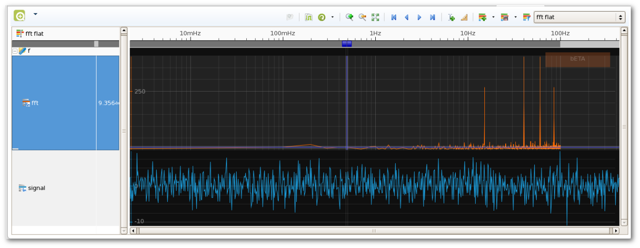
After opening a file tracer (Impulse.open('fft.trace'), it adds two signals, signal (time domain) and fft (frequency domain). Then it writes the content using the writeFloat method. That's it !

A03 recTr Trace Record Format

---